
2021. 4. 28. 00:24ㆍPython/문법
Ver. Jupyter Notebook (Anaconda3)
▶ pandas
● 데이터 유형
- 1차원(Series) : 한 줄 (행or열)
- 2차원(Dataframe) : 두 줄 (행, 열)
import pandas as pd		# 시리즈, 데이터프레임 데이터분석 라이브러리
import numpy as np		# 숫자, 행렬 라이브러리
▶ Series: 1차원 데이터
- A one-dimensional labeled array capable of holding any data type
s = pd.Series([3, -5, np.nan, 4], index=['a', 'b', 'c', 'd'])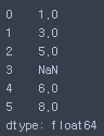
▶ DataFrame (2차원 데이터)
- A two-dimensional labeled data structure with columns of potentlally different tpes
● Object creation
- 날짜
dates = pd.date_range('20130101', periods=6, freq='D') # freq= Y:년, M:월, D:일
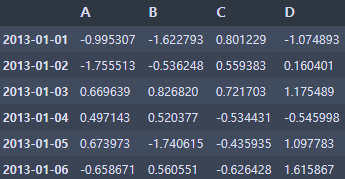
- 데이터프레임-1
df = pd.DataFrame(np.random.randn(6, 4), index=dates, columns=list('ABCD'))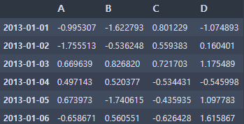
- 데이터프레임-2
df2 = pd.DataFrame({'A':1,
                   'B':pd.Timestamp('210427'),
                   'C':pd.Series(1, index=list(range(4)), dtype='float'),
                   'D':np.array([3]*4, dtype='int'),
                   'E':pd.Categorical(["test", "train", "test", "train"]),
                   'F':'foo'})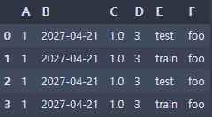
- 데이터 정보 (널값 확인)
df2.info()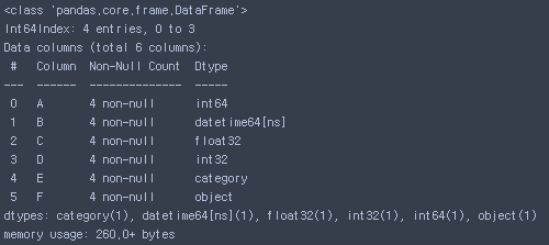
- 데이터 타입
df.dtypes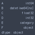
● Viewing data
- 행, 열 개수
df.shape
- 행 상위 개수
df.head(10)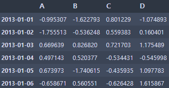
- 행 하위 개수
df.tail(3)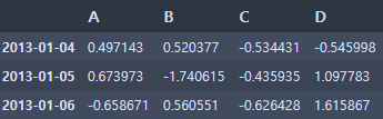
- 행 목록
df.index
- 열 목록
df.columns
- values 목록
df.values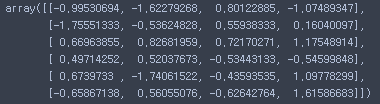
- 행, 열 바꾸기
dt.T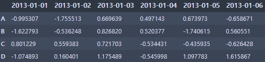
- 행/열 오름차순/내림차순 정렬
# axis= 0:index, 1:columns / ascending= Turn:내림차순, False:오름차순
df.sort_index(axis=1, ascending=False)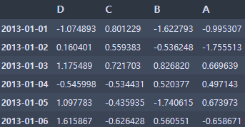
- 데이터 내림차순 정렬
df.sort_values(by='B', ascending=False)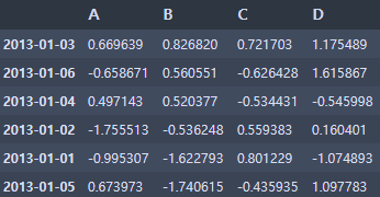
● Selection
# Getting
- 특정 열 선택
df['A']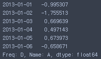
- 행 선택(범위)
df[0:3]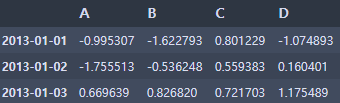
- 행 선택 (이름)
df['20130104':'20130106']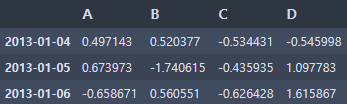
# Selection by label : loc[]
dates
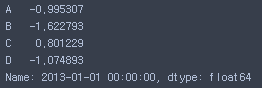
- loc[] : 이름으로 선택
df.loc[dates[0]]
df.loc[:, ['A', 'B']]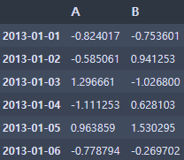
df.loc['20130102':'20130104', 'A':'C']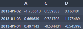
df.loc[dates[0], 'A']
# Selection by positionl : iloc[]
- iloc[] : 범위로 선택
df.iloc[3]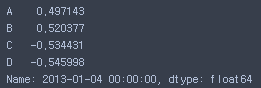
df.iloc[[1, 2, 4], [3, 2]]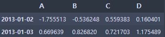
df.iloc[1:3, :]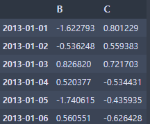
# 조건에 맞는 값 가져오기 (Boolean indexing)
df[df['A'] > 0]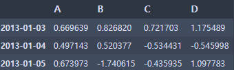
df[df > 0]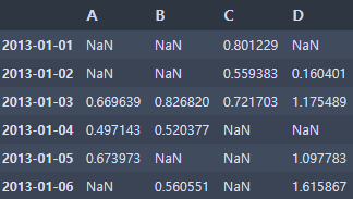
- 열 추가
df2['E'] = ['one', 'one', 'two', 'three', 'four', 'three']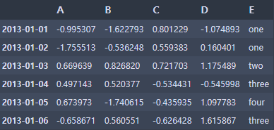
# 데이터의 특정 값 선택 (isin: is in(들어있는))
df2[df2['E'].isin(['two', 'four'])] 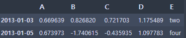
# Setting
- 행 데이터 추가
s1 = pd.Series([1, 2, 3, 4, 5, 6], index=pd.date_range('20130102', periods=6))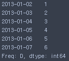
df['F'] = s1
df.loc[dates[0], 'A'] = 0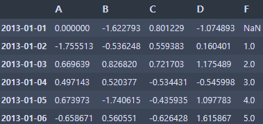
df.iloc[0,1]=0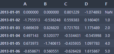
na.array([5] * len(df))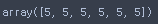
df.loc[:, 'D'] = np.array([5] * len(df))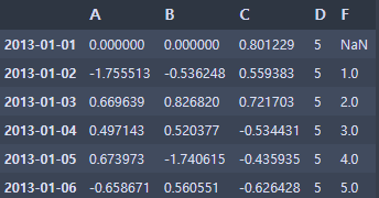
- df2의 0보다 큰 값들은 마이너스를 곱하라
df2 = df.copy()
df2[df2 > 0] = -df2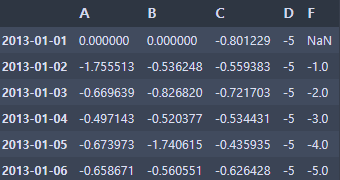
● Missing data
pandas primarily uses the value np.nan to represent missing data.
It is by default not included in computations.
df1 = df.reindex(index=dates[0:4], columns=list(df.columns) + ['E'])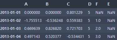
df1.loc[dates[0]:dates[1], 'E'] = 1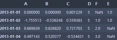
- NaN값이 있는 행들은 모두 삭제
df1.dropna(how='any')
- NaN값이 있는 자리에 value를 채우기
df1.fillna(value=5)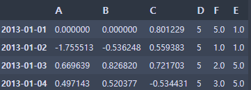
- NaN값이 있는지 확인하기
df1.isna(df1)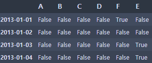
df1.isna().sum()
df1.isna().sum().sum()
● Operations
# Stats(통계 데이터)
Operations in general exclude missing data.
Performing a descriptive statistic:
- 평균 값
# 0: 열별로 평균, 1: 행별로 평균
df1.mean(0)
df1.mean(1)
- 이동
s = pd.Series([1, 3, 5, np.nan, 6, 8], index=dates)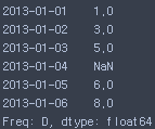
s = pd.Series([1, 3, 5, np.nan, 6, 8], index=dates),shift(2)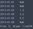
df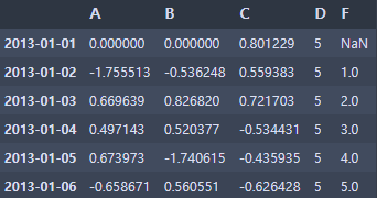
- 빼기
# df의 각 값들에서 s를 뺀다
# sub: 빼다(마이너스)
df.sub(s, axis='index')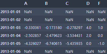
- 평균 값 등...
df.describe()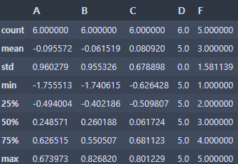
# Apply
df
- 누적 합계(밑으로 누계)
df.apply(np.cumsum)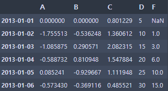
- 각 열마다 최대값-최소값
pf.apply(lambda x: x.max() - x.min()))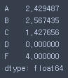
# Histogramming
s = pd.Series(np.random.randint(0, 5, size=10))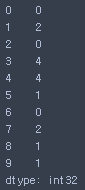
- 데이터 카운트
s.value_counts()
# String Methods
s= pd.Series(['A', 'B', 'C', 'Aaba', 'Baca', np.nan, 'CABA', 'dog', 'cat'])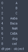
- 소문자로 바꾸기
s.str.lower()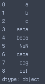
● Merge
# Concat (위 아래로 붙이는것)
df = pd.DataFrame(np.random.randn(10, 4))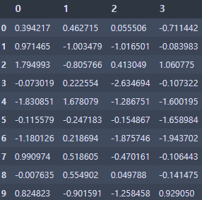
- 행렬 조각내기
pieces = [df[:3], df[3:7], df[7:]]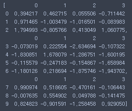
- 조각난 데이터 다시 행렬로 바꾸기
pd.concat(pieces)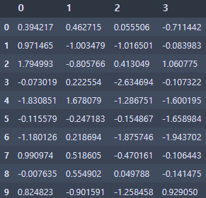
# merge
left = pd.DataFrame({'key': ['foo', 'foo'], 'lval': [1, 2]})
right = pd.DataFrame({'key': ['foo', 'foo'], 'lval': [4, 5]})
pd.merge(left, right, on='key')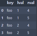
left = pd.DataFrame({'key': ['foo', 'bar'], 'lval': [1, 2]}) 
right = pd.DataFrame({'key': ['foo', 'bar'], 'lval': [4, 5]})
pd.merge(left, right, on='key')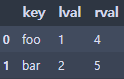
● Grouping
- groupby
df = pd.DataFrame({'A': ['foo', 'bar', 'foo', 'bar',
                          'foo', 'bar', 'foo', 'foo'],
                   'B': ['one', 'one', 'two', 'three',
                          'two', 'two', 'one', 'three'],
                   'C': np.random.randn(8),
                   'D': np.random.randn(8)}
                 )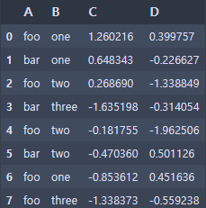
df.groupby('A').sum()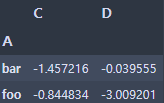
df.groupby(['A', 'B']).sum()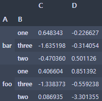
● Reshaping
# stack
tuples = list(zip(*[['bar', 'bar', 'baz', 'baz',
                     'foo', 'foo', 'qux', 'qux'],
                    ['one', 'two', 'one', 'two',
                     'one', 'two', 'one', 'two']]))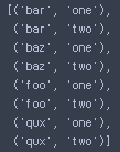
index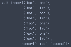
df = pd.DataFrame(np.random.randn(8, 2), index=index, columns=['A', 'B'])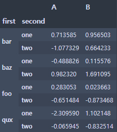
df2 = df[:4]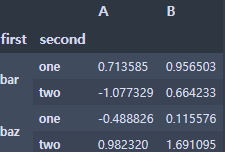
- stack()을 하면 데이터를 쌓아서 보여줌
stacked = df2.stack()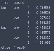
- unstack()를 하면 원상복귀
stacked.unstack()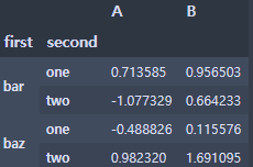
# Pivot tables (기준 테이블)
df = pd.DataFrame({'A': ['one', 'one', 'two', 'three'] * 3,
                   'B': ['A', 'B', 'C'] * 4,
                   'C': ['foo', 'foo', 'foo', 'bar', 'bar', 'bar'] * 2,
                   'D': np.random.randint(0, 11, size=12),
                   'E': np.random.randint(0, 11, size=12)})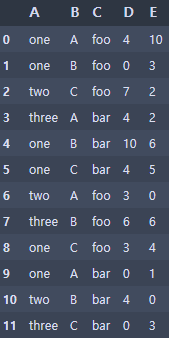
pd.pivot_table(df, values=['D', 'E'] , index=['A', 'B'], columns=['C'])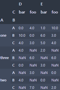
▶ 엑셀 다루는 판다스
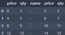
● 새 column 추가하기
- reshape : 행렬처럼
df = pd.DataFrame(np.arange(16).reshape(4,4),
                  index=None,
                  columns=['price', 'qty', 'price', 'qty'])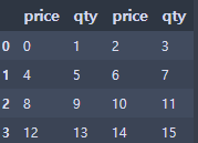
df['name'] = '-'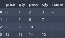
● 원하는 위치에 column 추가하기
df = pd.DataFrame(np.arange(16).reshape(4,4),
                  index=None,
                  columns=['price', 'qty', 'price', 'qty'])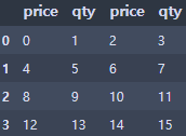
- df.insert(loc, column, value, allow_duplicates=Ture or False)
df.insert(2, 'name', '-', allow_duplicates=False)
● 기본 테이블을 멀티 column, index로 바꾸기
df1 = pd.DataFrame(np.arange(16).reshape(4,4),
                  index=None,
                  columns=['price', 'qty', 'price', 'qty'])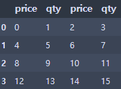
df2 = pd.DataFrame(df1.values,
                   index = df1.index,
                   columns = [['apple','apple','banana','banana'], ['price','qty','price','qty']])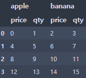
● 이름으로 행, 열 삭제
df = pd.DataFrame(np.arange(16).reshape(4,4),
                  index=None,
                  columns=['price', 'qty', 'price', 'qty'])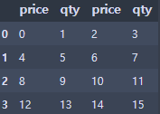
df = df.drop(['price'], axis=1)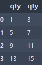
df = df.drop([2], axis=0)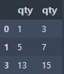
● n번째 행 삭제
df1 = pd.DataFrame(np.arange(16).reshape(4,4),
                  index=None,
                  columns=['price', 'qty', 'price', 'qty'])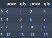
df2 = df1.drop(df1.index[0], axis=0)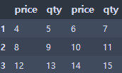
● 마지막 행에 cloumn 별 합계 삽입
df = pd.DataFrame(np.arange(6).reshape(2,3),
                  index=None,
                  columns=['price', 'qty', 'like'])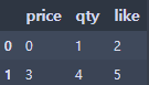
df.loc['합계'] = [df[df.columns[x]].sum() for x in range(0, len(df.columns))]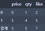
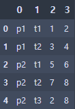
● 튜플을 데이터프레임으로 만들기
data = [
('p1', 't1', 1, 2),
('p1', 't2', 3, 4),
('p2', 't1', 5, 6),
('p2', 't2', 7, 8),
('p2', 't3', 2, 8)
]

df = pd.DataFrame(data)
'Python > 문법' 카테고리의 다른 글
| [python] kaggle, boston marathon (0) | 2021.04.29 |
|---|---|
| [python] 외부데이터 (0) | 2021.04.29 |
| [Python] 정리 (0) | 2021.04.29 |
| [python] 심화 (0) | 2021.04.27 |
| [python] 기초 (0) | 2021.04.27 |